PostgreSQL Query Planning and Execution Engine: A Beginner’s Guide

Introduction

Imagine you’re planning a road trip. You’d probably:

1. Look at a map to find different routes
2. Consider factors like traffic, distance, and road conditions
3. Choose the most efficient path
4. Follow that path to reach your destination

PostgreSQL does something remarkably similar when executing your SQL queries. This process—query planning and execution—is fundamental to database performance, yet it often remains a mystery to many database users.

In this post, we’ll pull back the curtain on PostgreSQL’s query planning and execution engine, explaining how it transforms your SQL into efficient operations that retrieve or modify your data.

Table of Contents

1. The Journey of a Query: A High-Level Overview
2. Query Planning: Finding the Best Route
   • Parsing and Analysis
   • Statistics and Cost Estimation
   • Plan Generation
3. Query Execution: Following the Map
   • Execution Tree
   • Access Methods
   • Join Algorithms
4. Understanding EXPLAIN: Reading the Map
   • Basic EXPLAIN Output
   • EXPLAIN ANALYZE
   • Interpreting Common Plan Operations
5. Common Performance Issues and Solutions
   • Missing Indexes
   • Suboptimal Join Orders
   • Statistics Problems
6. Advanced Topics
   • Parallel Query Execution
   • JIT Compilation
   • Custom Plans vs. Generic Plans
7. Conclusion

The Journey of a Query: A High-Level Overview

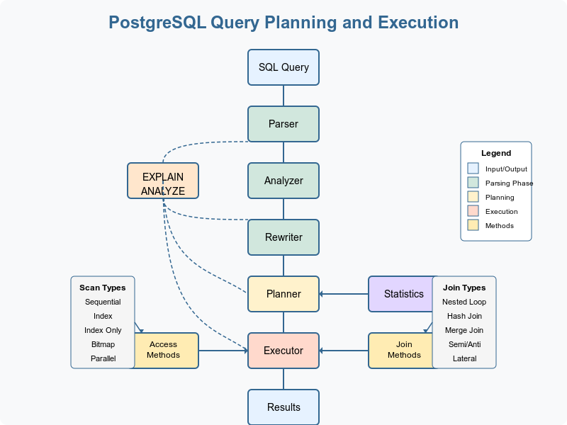
When you send a SQL query to PostgreSQL, it doesn’t immediately start fetching or modifying data. Instead, it follows a sophisticated process:

1. Parse the SQL text into an internal representation
2. Analyze this representation to ensure it makes sense
3. Rewrite the query if needed (for views, rules, etc.)
4. Plan the most efficient execution strategy
5. Execute the plan to produce results

Think of it like a GPS navigation system—it doesn’t just blindly follow the first path it finds. It analyzes traffic conditions, calculates multiple routes, and then chooses the most efficient one.

Query Planning: Finding the Best Route

Parsing and Analysis

When you write a SQL query like:

SELECT customers.name, orders.order_date 
FROM customers 
JOIN orders ON customers.id = orders.customer_id
WHERE orders.total > 100;

PostgreSQL first parses this text into a tree structure that represents the query’s logical meaning. During analysis, it:

• Verifies that tables and columns exist
• Checks that data types are compatible
• Resolves column names and aliases
• Ensures you have the necessary permissions

Think of this stage like checking that your destination exists and that all the roads on your map are actually real roads.

Statistics and Cost Estimation

To choose the best execution plan, PostgreSQL relies on statistics about your data. These statistics, collected by the ANALYZE command, include:

• Number of rows in each table
• Number of distinct values in each column
• Most common values in each column
• Data distribution

With these statistics, PostgreSQL estimates the “cost” of different operations. Cost is a unitless measure that combines:

• CPU time (processing effort)
• I/O time (disk access)
• Memory usage

Imagine you’re deciding between two routes—one is shorter but has heavy traffic, while another is longer but moves faster. PostgreSQL makes similar trade-offs.

Plan Generation

PostgreSQL’s query planner evaluates many possible execution strategies:

• Different join orders (which table to access first)
• Different join methods (nested loop, hash join, merge join)
• Different scan methods (sequential scan, index scan)
• Whether to use sorting or hashing for operations

For example, when joining customers and orders, PostgreSQL might consider:

1. Scanning all customers, then finding matching orders for each
2. Scanning all orders, then finding the corresponding customer
3. Building a hash table of customers, then probing it with orders
4. Sorting both tables and performing a merge join

The planner calculates the estimated cost for each approach and selects the plan with the lowest total cost.

Query Execution: Following the Map

Execution Tree

The selected plan forms an execution tree—a hierarchy of operations where the output of lower operations feeds into higher ones.

Consider our example query:

SELECT customers.name, orders.order_date 
FROM customers 
JOIN orders ON customers.id = orders.customer_id
WHERE orders.total > 100;

A simplified execution tree might look like:

Project (output name and order_date)
  └─ Hash Join (customers.id = orders.customer_id)
      ├─ Seq Scan on customers
      └─ Hash
          └─ Filter (orders.total > 100)
              └─ Seq Scan on orders

Reading from bottom to top:

1. Scan the orders table
2. Filter for orders with total > 100
3. Build a hash table from these orders
4. Scan the customers table
5. For each customer, probe the hash table to find matching orders
6. Output the name and order_date for matching pairs

Access Methods

PostgreSQL offers several ways to access data:

Sequential Scan: Reads the entire table, row by row. Like reading a book from start to finish.

Seq Scan on customers

Index Scan: Uses an index to find specific rows. Like using a book’s index to jump to relevant pages.

Index Scan using orders_customer_id_idx on orders

Index Only Scan: Retrieves data directly from the index without touching the table. Like a book’s index that contains all the information you need.

Index Only Scan using customers_name_idx on customers

Bitmap Scan: Uses an index to create a bitmap of matching rows, then retrieves them all at once. Useful for retrieving a moderate number of rows.

Bitmap Heap Scan on orders
  └─ Bitmap Index Scan on orders_total_idx

Join Algorithms

When combining data from multiple tables, PostgreSQL can use different join methods:

Nested Loop Join: For each row in one table, scan the other table for matches. Efficient when one table is small and the other has an index on the join column.

Nested Loop
  ├─ Seq Scan on small_table
  └─ Index Scan on big_table

Hash Join: Build a hash table from one table, then probe it with rows from the other table. Good for large tables without useful indexes.

Hash Join
  ├─ Seq Scan on customers
  └─ Hash
      └─ Seq Scan on orders

Merge Join: Sort both tables on the join column, then merge them like a zipper. Efficient when both tables are already sorted.

Merge Join
  ├─ Sort
  │   └─ Seq Scan on customers
  └─ Sort
      └─ Seq Scan on orders

Understanding EXPLAIN: Reading the Map

PostgreSQL’s EXPLAIN command reveals the execution plan for a query without actually executing it.

Basic EXPLAIN Output

EXPLAIN SELECT * FROM customers WHERE city = 'New York';

Might produce:

                        QUERY PLAN
----------------------------------------------------------
 Seq Scan on customers  (cost=0.00..22.00 rows=20 width=80)
   Filter: ((city)::text = 'New York'::text)

This tells us PostgreSQL will:

1. Perform a sequential scan of the customers table
2. Filter rows where city equals ‘New York’
3. Estimated cost starts at 0.00 and ends at 22.00
4. Expects to return approximately 20 rows
5. Each row is approximately 80 bytes wide

EXPLAIN ANALYZE

Adding ANALYZE actually executes the query and shows both the plan and actual results:

EXPLAIN ANALYZE SELECT * FROM customers WHERE city = 'New York';

Output:

                                   QUERY PLAN
----------------------------------------------------------------------------------
 Seq Scan on customers  (cost=0.00..22.00 rows=20 width=80)
                        (actual time=0.020..0.148 rows=18 loops=1)
   Filter: ((city)::text = 'New York'::text)
   Rows Removed by Filter: 982
 Planning Time: 0.065 ms
 Execution Time: 0.174 ms

Now we see:

1. The query actually returned 18 rows (close to the estimate of 20)
2. It took 0.148 milliseconds to complete the scan
3. 982 rows were examined but didn’t match the filter
4. Planning took 0.065 ms and execution took 0.174 ms

Interpreting Common Plan Operations

Here are some common operations you’ll see in EXPLAIN output:

• Seq Scan: Full table scan
• Index Scan: Using an index to access the table
• Bitmap Scan: Two-phase approach using an index to build a bitmap, then accessing the table
• Nested Loop/Hash Join/Merge Join: Different join algorithms
• Sort: Sorting data (usually for ORDER BY, GROUP BY, or certain joins)
• Aggregate: Computing aggregate functions (COUNT, SUM, AVG, etc.)
• Limit: Restricting the number of returned rows

Common Performance Issues and Solutions

Missing Indexes

Problem: Sequential scans on large tables when filtering or joining.

Example EXPLAIN output:

Seq Scan on large_orders  (cost=0.00..12432.00 rows=50 width=80)
  Filter: (customer_id = 12345)

Solution: Create an index on the filtered or join column.

CREATE INDEX large_orders_customer_id_idx ON large_orders(customer_id);

After creating the index:

Index Scan using large_orders_customer_id_idx on large_orders  (cost=0.42..8.44 rows=50 width=80)
  Index Cond: (customer_id = 12345)

Suboptimal Join Orders

Problem: PostgreSQL joining tables in a non-optimal order.

Example:

Hash Join  (cost=1.09..13520.00 rows=1000 width=16)
  Hash Cond: (large_table.small_id = small_table.id)
  -> Seq Scan on large_table  (cost=0.00..10000.00 rows=100000 width=12)
  -> Hash  (cost=1.08..1.08 rows=100 width=4)
      -> Seq Scan on small_table  (cost=0.00..1.08 rows=100 width=4)

Solution: Increase random_page_cost for SSDs or adjust join_collapse_limit for complex queries.

Statistics Problems

Problem: PostgreSQL making poor decisions due to outdated or insufficient statistics.

Solution: Run ANALYZE to update statistics or adjust sampling rate for better accuracy.

ANALYZE large_table;
-- Or with increased sampling
ALTER TABLE large_table ALTER COLUMN complex_column SET STATISTICS 1000;
ANALYZE large_table;

Advanced Topics

Parallel Query Execution

PostgreSQL can divide work across multiple CPU cores:

Gather  (cost=1000.00..12432.00 rows=1000 width=80)
  Workers Planned: 2
  ->  Parallel Seq Scan on large_table  (cost=0.00..10432.00 rows=500 width=80)

To enable or adjust parallel behavior:

SET max_parallel_workers_per_gather = 4;

JIT Compilation

For complex queries, Just-In-Time compilation can improve performance:

SET jit = on;
SET jit_above_cost = 100000;

Custom Plans vs. Generic Plans

For prepared statements, PostgreSQL can use:

• Custom plans: Optimized for specific parameter values
• Generic plans: Reusable across different parameter values

Control with:

SET plan_cache_mode = 'force_custom_plan';
-- or
SET plan_cache_mode = 'force_generic_plan';

Conclusion

Understanding PostgreSQL’s query planning and execution engine gives you powerful insights into database performance. By learning to “read the map” with EXPLAIN, you can identify bottlenecks, optimize indexes, and tune your database for peak efficiency.

Remember that query planning is a complex process with many factors:

• Table statistics
• Index availability
• Data distribution
• Configuration parameters
• Query complexity

When performance matters, don’t guess—use EXPLAIN ANALYZE to see exactly what PostgreSQL is doing with your queries.

Like any journey, reaching your destination efficiently requires knowing the territory and choosing the right path. With the knowledge from this guide, you’re now better equipped to navigate the PostgreSQL performance landscape.

Happy querying!